[Paper Review] Revolution and peak discrepancy-based domain alignment method for bearing fault diagnosis under very low-speed conditions

The first paper I will review is ‘Revolution and Peak Discrepancy-Based Domain Alignment Method for Bearing Fault Diagnosis Under Very Low-Speed Conditions’ written by Ph.D. candidate Seungyun Lee from SNU HAI Lab.

> 1. Introduction

VLS (Very-Low-Speed) bearings typically operate at speeds below 10 RPM. They are mainly installed in large mechanical systems, such as wind turbines and radar systems, where they support substantial weight. Due to the nature of these large-scale systems, diagnosing VLS bearings is crucial, as bearing failures can lead to severe accidents.

Unlike general bearings, VLS bearings have unique characteristics when it comes to fault diagnosis. Their operating speed is much slower, making fault signal analysis more challenging and resulting in weaker contact of the defective parts. The large scale of these systems can also lead to the generation of significantly different characteristic frequencies, which are essential for diagnosing bearing faults.

Previous studies have attempted to align different domains for bearing fault diagnosis but have not considered the differences in operating conditions and scales of the bearing systems. Such approaches tend to focus on developing neural network architectures or loss functions without quantifying the differences in fault signals caused by variations in rotational speed conditions and the geometric features of the bearings. To successfully perform transfer learning (TL) between general bearings and VLS bearings, an approach that quantifies and aligns domain differences while considering the physical knowledge of the bearing system should be employed. Therefore, this paper proposes a novel domain alignment framework that reflects the physical characteristics of VLS bearings, which can be used for TL from high-speed to VLS bearings.

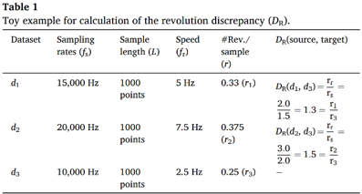
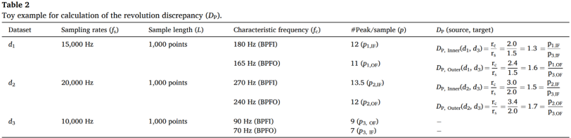
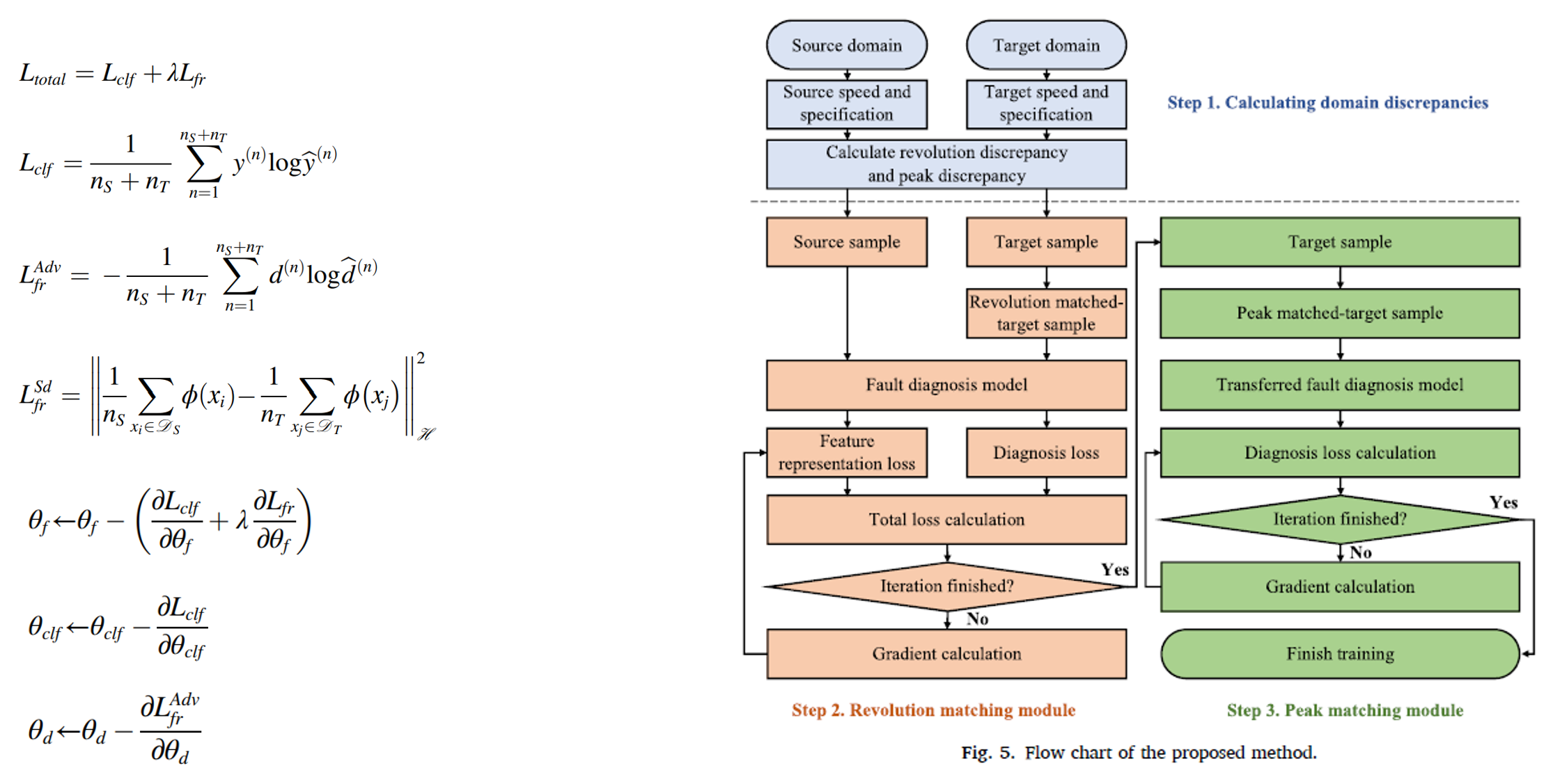
> 2. Proposed Method 1: Discrepancy Quantification

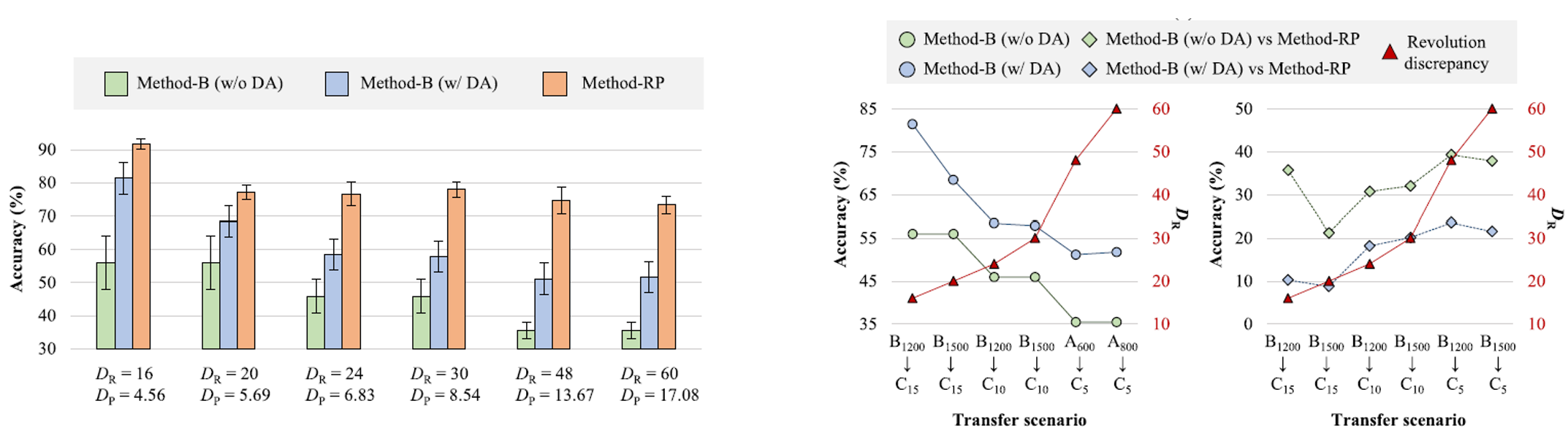
The first proposal in this paper is the quantification of the domain discrepancy between bearings operating at different speeds. This includes the Revolution Discrepancy Metric and the Peak Discrepancy Metric, with the equations provided below. Through the examples in Table 1 and 2, it can be understood that as the discrepancy between domains increases, the Revolution Discrepancy also increases.

> 2. Proposed Method 2: Revolution matching module (RMM)

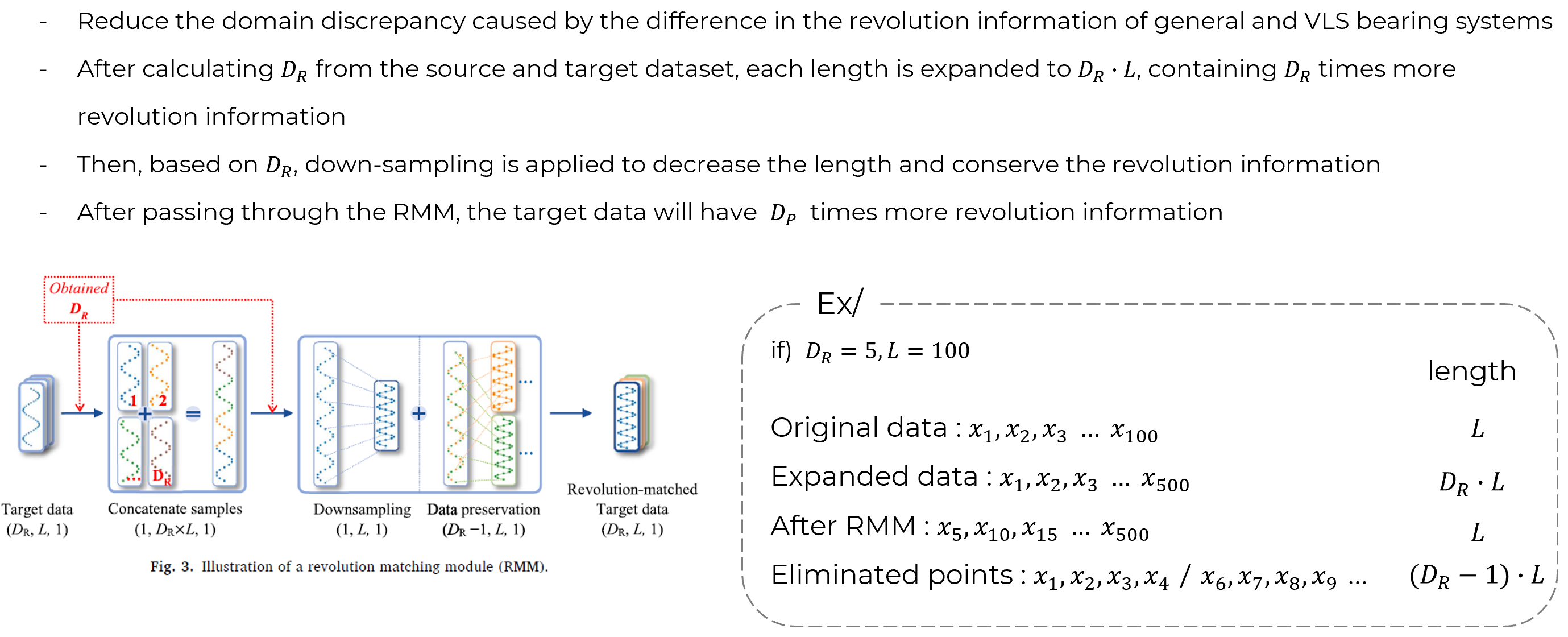
After downsampling, the remaining data length is L, which may lead to a reduction in data quantity to 1/DR. This reduction could pose a problem, as it contradicts the goal of TL, which aims to solve tasks under limited data conditions. To address this issue, a preservation process is carried out after the Revolution Discrepancy Metric (RMM).

Let’s consider an example (see dotted Ex/ box). If DR=5 and L=100, the original data consists of a sequence of 1, 2, 3… up to a length of L. The expanded data, having been multiplied by DR, extends up to 500. After passing through RMM, the remaining data has a length of L, but since every 5th data point was selected, it consists of 5, 10, 15… up to 100 points. The removed points would be 1, 2, 3, 4 / 6, 7, 8, 9, and so on, resulting in (DR-1) sets of removed samples with a length of L. By using these removed sample sets as training data, data preservation is achieved.

> 2. Proposed Method 3: Peak matching module (PMM)

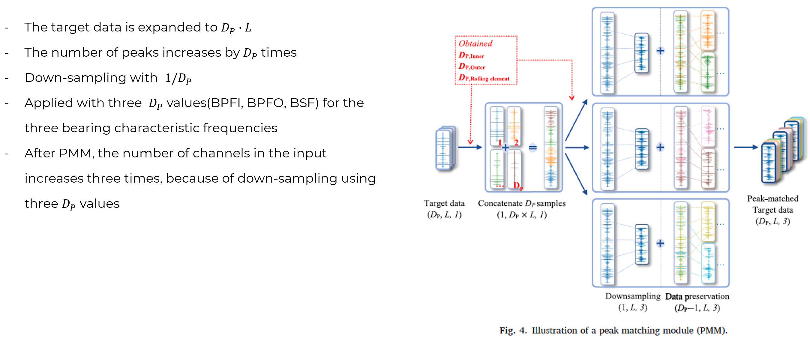
There is a difference between DP and DR, where DP consists of multiple values along with bearing characteristic frequencies, while DR is defined as a single value. DP is applied to the three values corresponding to the three bearing characteristic frequencies (BPFI, BPFO, BSF). This approach is necessary because the labels of the target data input to the DL model during the PMM process cannot yet be identified. As a result of PMM, the number of peaks matches, and the length of the samples becomes equal to L. After PMM, the only difference in input dimensions is that the number of channels increases threefold due to downsampling. Additionally, the data preservation performed in RMM is also applied to the peak-matched data, maintaining the data quantity.

> 2. Proposed Method : Training Strategy

> 3. Experimental Validation: Setup

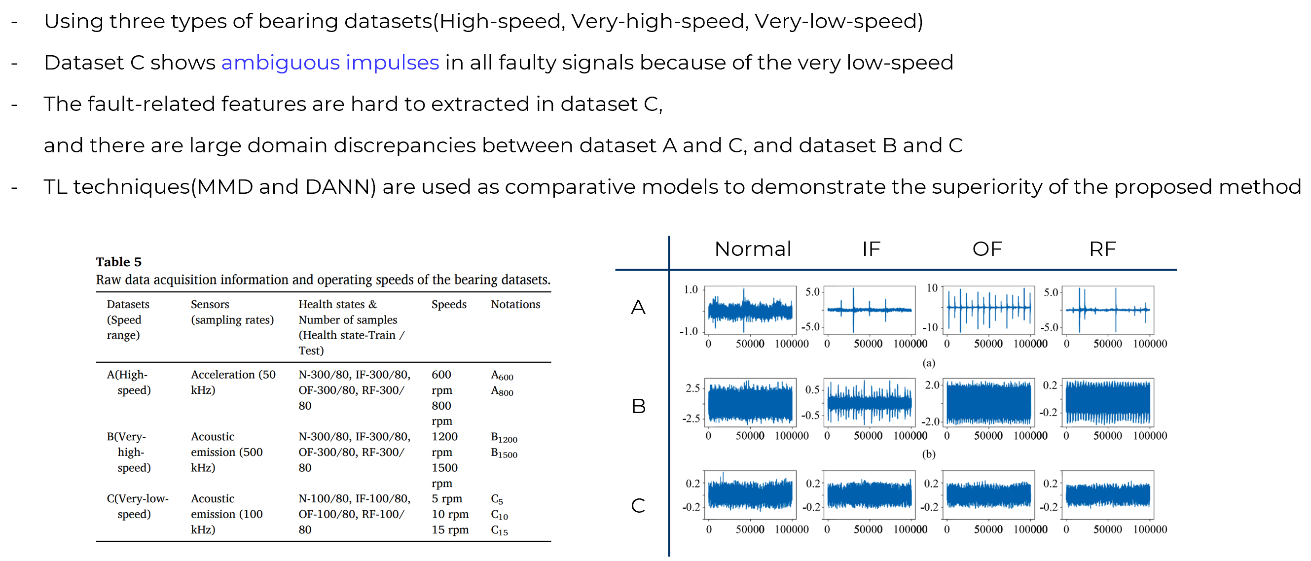
Looking at normal bearings and the most common faults that occur during bearing use, such as inner, outer, and rolling element faults, the impulse signals are clearly visible in high-speed and ultra-high-speed bearings, but they are relatively difficult to detect in VLS bearings. Therefore, it is challenging to extract fault-related features from Dataset C, and there is a significant domain discrepancy between Dataset A and C, as well as between Dataset B and C.

To demonstrate the superiority of the proposed method, we use two representative TL methods, MMD and DANN, as comparison models.

> 3. Experimental Validation: Results for applying RMM and PMM

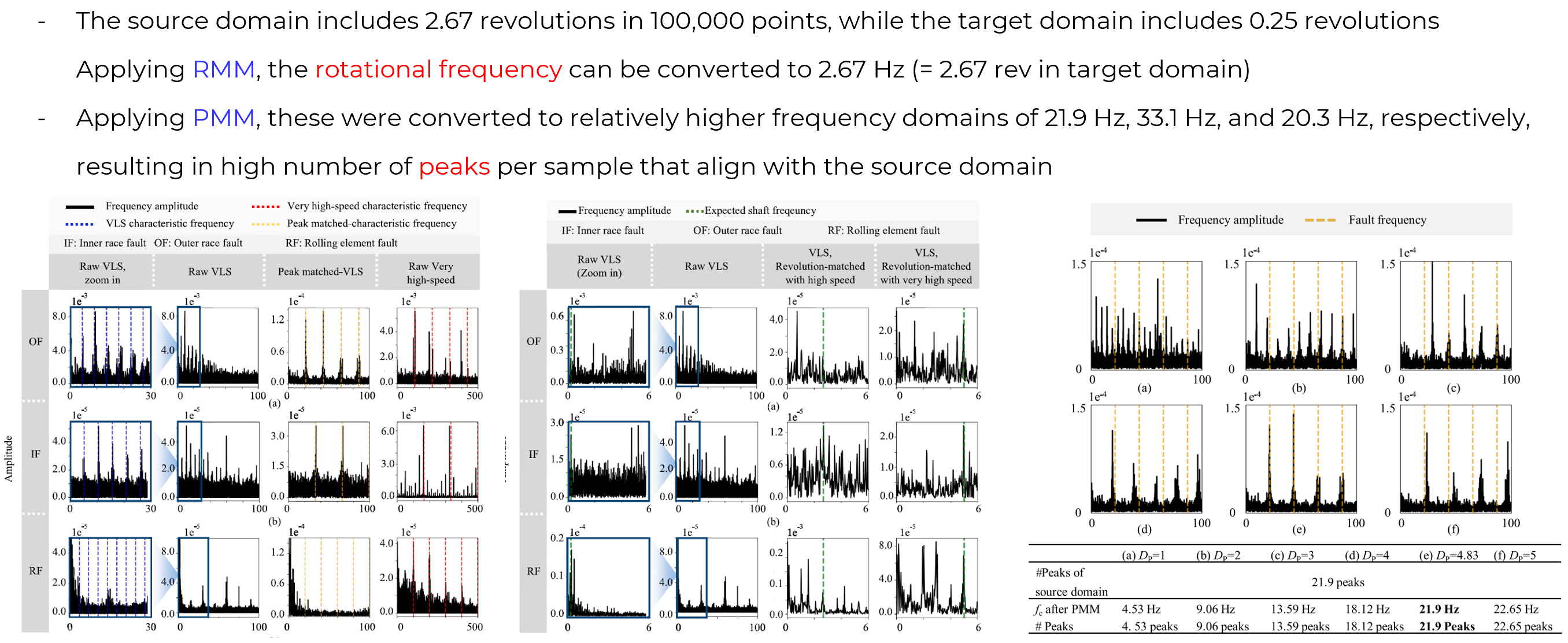
We analyze the results of RMM and PMM using Fast Fourier Transform. In this context, the source domain data theoretically includes 2.67 revolutions within 100,000 sample points. However, the target domain data, before applying RMM, includes only 0.25 revolutions. After applying RMM, the rotational frequency can be adjusted to 2.67 Hz, which corresponds to 2.67 revolutions in the target domain. Similarly, after applying PMM, the number of high peaks aligns with those in the source domain. As shown in the figure on the right, when PMM is applied using the correct DP values, the number of peaks most closely matches those in the source domain.

> 3. Experimental Validation: Case Study

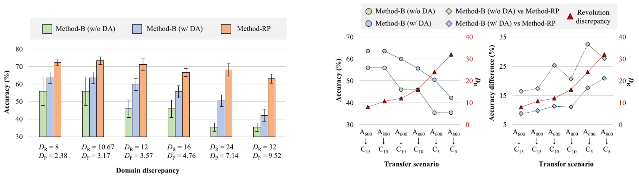Case Study 1

Case Study 2

In the first case study, we compared TL from Dataset A to C, and in the second case study, TL from Dataset B to C. As shown in the figure on the right, the proposed model exhibits relatively stable accuracy even with large DR and DP values. As expected, in cases of significant domain discrepancies, there is a considerable difference in accuracy between the baseline model and the proposed model. When DR increases by the same amount, the proposed model’s accuracy decreases by only 10.20%, whereas the baseline model’s accuracy drops by 21.38%. This indicates that DR and DP can effectively quantify domain differences, and applying RMM and PMM can reduce these differences.

A notable observation from the results of the two case studies is that, despite having lower DR and DP values, the TL accuracy from high-speed to VLS is lower than that from ultra-high-speed to VLS. The reasons for this are twofold. First, in the case of Dataset A, acceleration signals were used to diagnose acoustic emission signals in the source domain, and there may be physical differences between the acceleration sensor and the AE sensor. Second, these results are due to differences in the domain between datasets and the speed conditions within the datasets.

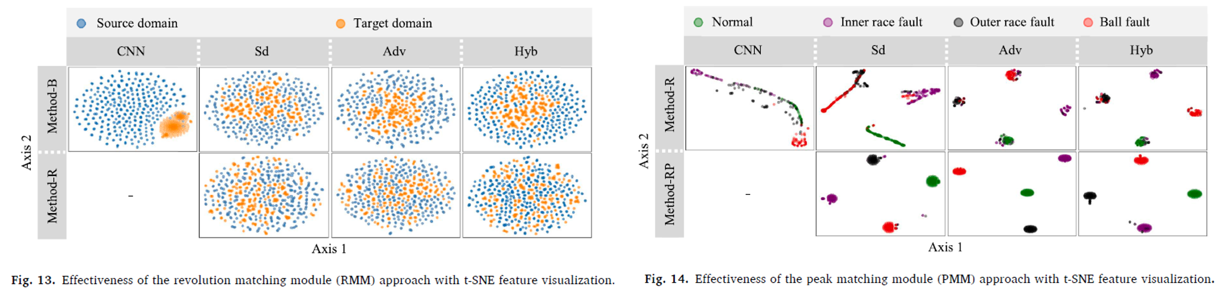
To clearly demonstrate the effects of RMM and PMM, feature visualization results are presented. The features of Sd-B, Adv-B, and Hyb-B can be distinguished between the two domains, with the source domain located on the outside and the target domain on the inside. However, the features of Sd-R, Adv-R, and Hyb-R are more challenging to separate into distinct domains compared to Method-B. This well-mixed appearance illustrates RMM’s ability to extract features independent of speed. PMM, on the other hand, enables differentiation according to each fault type. Representations without PMM show ambiguous clusters for each fault type, whereas the results with PMM demonstrate more clearly separated features. Despite some minor errors, distinct clusters for each fault type are clearly formed.

4. Conclusion

The paper proposed the Revolution and Peak Discrepancy Metrics, Revolution Matching Module, and Peak Matching Module. By applying them to three different bearing datasets and comparing the results with previous approaches, the proposed methods improved the average accuracy by 20.72% in the scenario with the largest domain discrepancy and by 18.88% under the most insufficient data condition.